
Table of Contents
Prediction
The aim of the Prediction tool is to take advantage of the signalling circuit activities to distinguish between phenotypes (a two group comparison).
HiPathia Prediction uses the signalling value of mechanism-based biomarkers to train a SVM prediction model with cross-validation-based techniques. Moreover, previously obtained models could be used to predict the phenotype of new samples.
The tool can be accessed from the main menu bar, by clicking on the Prediction button, see Workflow for further information.
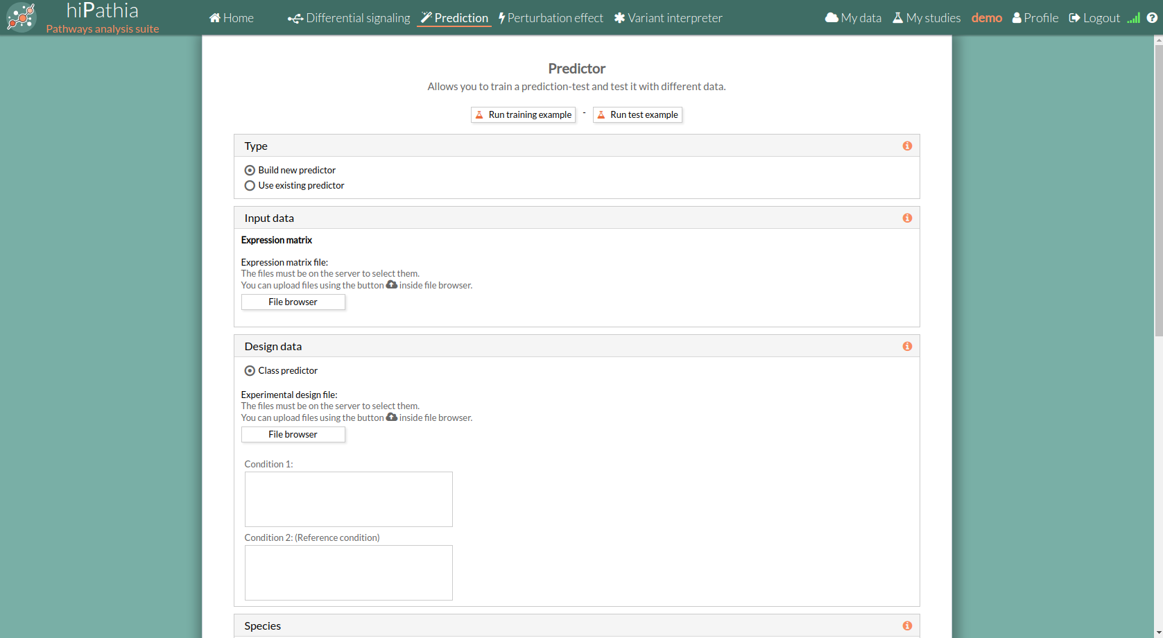
Prediction form
The main page of the tool is its filling form. This form includes all the information and parameters that the tool needs to process a study. The form is divided into different panels:
Type panel
The type panel allows you to choose the kind of prediction analysis you want to perform. You can choose between two options:
- Build new predictor: Train new prediction model with your selected data.
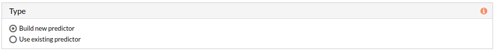
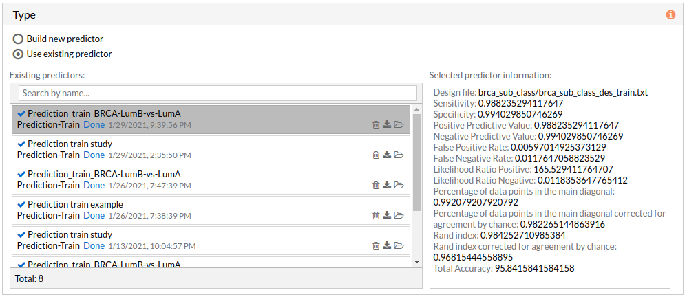
- Use existing predictor: Test existing model choosing an already trained model to predict the phenotype of new samples. Existing prediction models can be selected from your project folders stored in HiPathia's server.
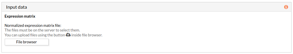
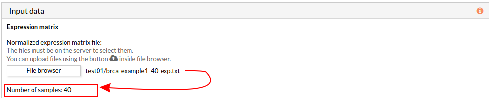
Input data panel
In the input data panel, we must introduce the expression data.
 The expression data has to be:
- Expression matrix provided by ourselves (see how to upload files in Upload your data).
When we select a gene expression file, the number of samples of this matrix will appear under the “file browser” button as shown below.
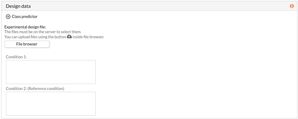
Design data panel (For training)
It will appear only if the Build new predictor is selected.
The design data panel allows you to choose the kind of experiment you want to perform:
- Two-Class predictor: The comparison is performed between the two classes described in the experimental design file.
The experimental design file must include two columns: the first one with the names of the samples, the second one with the class to which each sample belongs.
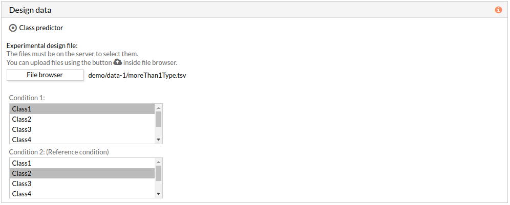
 If the experimental design file contains more than two classes then you have to select the appropriate class for each condition.
Note: condition 2 will be taken as a reference condition.
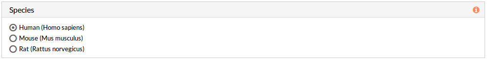
Species (For training)
Here we must choose the species of our experiment. You can choose among:
- Human (Homo sapiens)
- Mouse (Mus musculus)
- Rat (Rattus norvegicus).
Experimental design (For training)
This panel includes further parameters necessary to run an analysis.
Rank and filter circuits: Check to obtain the circuits that best differentiate your phenotype. This option is only available for the Build new predictor type.

Pathways
This panel includes the list of all available pathways in HiPathia. We can select the pathways with which the analysis will be performed.
HiPathia retrieves pathway information from KEGG database. KEGG pathway database is a collection of manually drawn pathway maps representing the knowledge on the molecular interaction, reaction and relation networks.
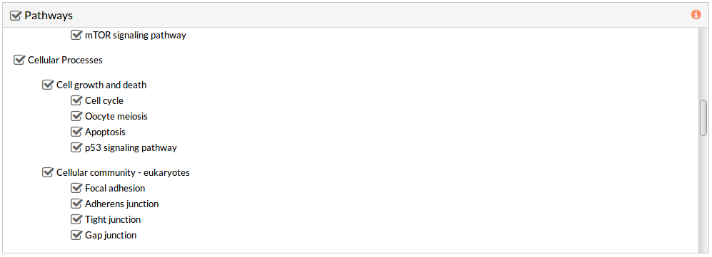 By default all available pathways are selected.
Note: At least one pathway has to be selected.
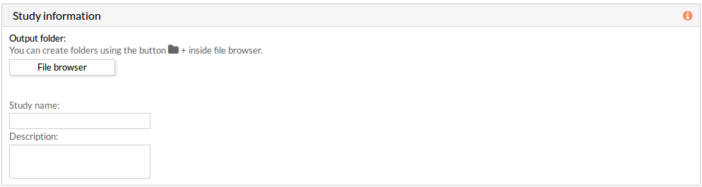
Study information
This panel includes some parameters in order to identify and save our study.
- Output folder: If we want to reorganize our studies we can select the folder in which we want save our report. By default the study will be saved in the home in a folder named “Prediction_train_study-N” if it is a training analysis or “Prediction_test_study-N” if it is a prediction test analysis, N is an integer number.
- Study name: We can give a name to our study. This is very useful to later identify it among the other studies listed in the My studies list.
The default study name is “Prediction_train_study-N” or Prediction_test_study-N“, N is an integer number. - Description: We can give a description to our study.
Run analysis
Once the form has been filled in, press the Run analysis button to launch the study.
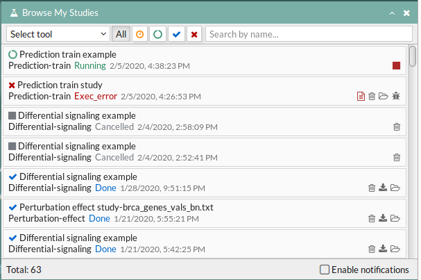
 Your study will be listed in the My studies panel, and a panel called Browse my studies will appear showing all your studies and their state. the new study will appear with a queued state then running state. If everything goes well, the state will be done after few minutes(depending on the inputs data and the availability of server).
All study states are:
Your study will be listed in the My studies panel, and a panel called Browse my studies will appear showing all your studies and their state. the new study will appear with a queued state then running state. If everything goes well, the state will be done after few minutes(depending on the inputs data and the availability of server).
All study states are:
- Queued: The information has been processed and the study has been sent and waits to be processed.
- Running: The study is in progress, study can be cancelled using the stop button.

- Done: The study has ended and the results are available to visualize and download.
- Cancelled: The study was canceled before finishing.
- Error: Sometimes a study can stop returning a error message, you can report and contact us in order to help you to fix it.

Training report
The report page of the Prediction tool includes different output results. You can download any table or image showed in the results page by clicking on the name right before it. You can also download the pathway and function matrices by clicking on Circuit values.
The results are divided in different panels:
Study Information
Here you can find the information about the selected study.
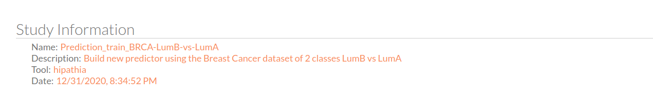
- Name: the study name.
- Description: the description of the current study.
- Tool: the name of the used tool (in this case, is Hipathia).
- Date: study's launching date (MM/DD/AAAA, HH:MM:SS AM/PM format)
Input Parameters
Here you can visualize the parameters with which the current study was launched.
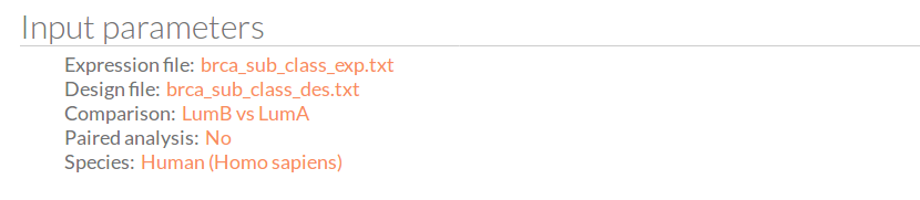
- Expression file: The name of the expression file that has been used in the current study.
- Design file: The name of the design file that has been used in the current study.
- Comparison: The groups that have been compared, for example; Normal vs Tumor.
- Paired analysis: Have the input data been paired? No or Yes.
- Species: The species of this experiment; Human (Homo sapiens),Mouse (Mus musculus) or Rat (Rattus norvegicus).
Circuit values
You can download the matrix of circuit activity values by clicking on circuit values.
 This matrix file indicates for each “effector circuit” the level of activation calculated using Hipathia method for each sample.
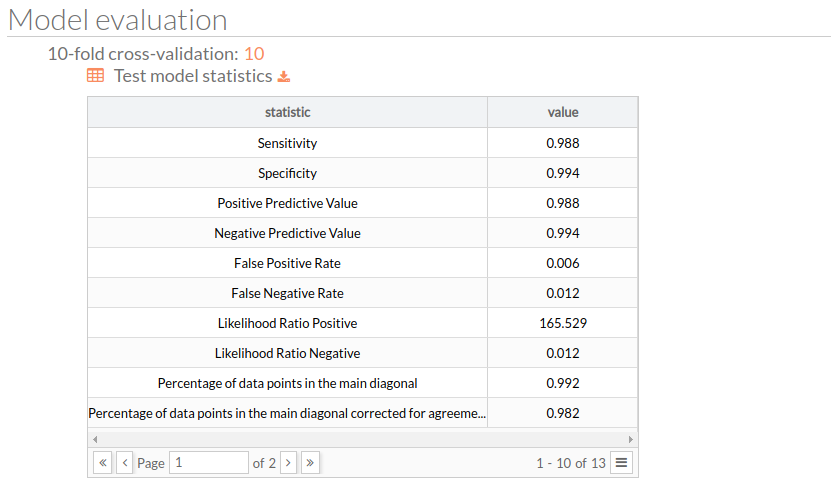
Model evaluation
Here you can visualize the results from the prediction analysis.
K-fold cross-validation
The number of equal-sized subsamples in which the original sample is randomly partitioned. Then a table for test model statistics is showed, each value represents the mean across the holdout folds for the corresponding metric or score:
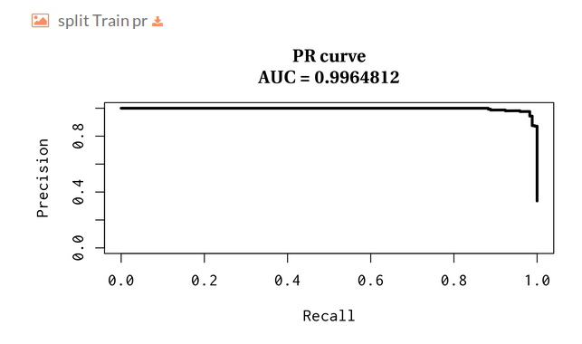
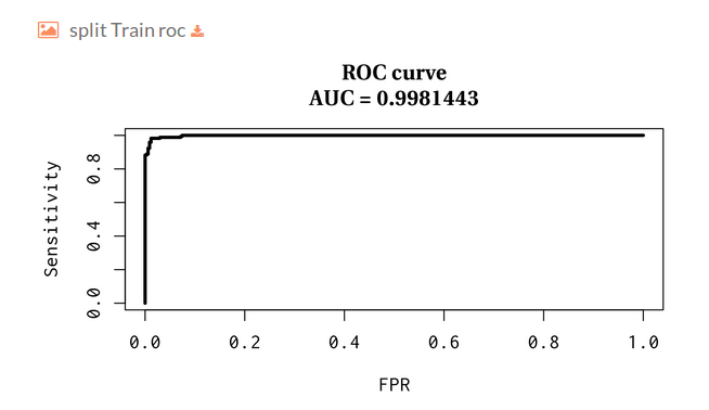
Validation of typical split
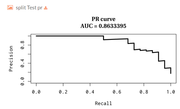
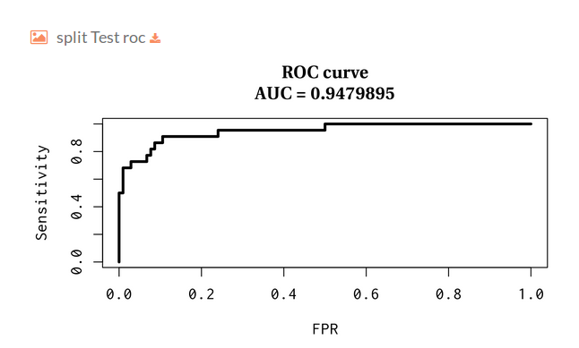
Then you will find several plots for train-test split validation, where we randomly holdout 30% of the data for the test while the remaining samples are used for training the model. The plots represent the receiver operating characteristic and precision and recall curves for each split.
- Split Train precision and recall:
- Split Train receiver operating characteristic:
- Split Test precision and recall:
- Split Test receiver operating characteristic:
Probability distribution
Here you can find a boxplot for the (predicted) probability distribution of the positive class over the test split with respect to the original labels:
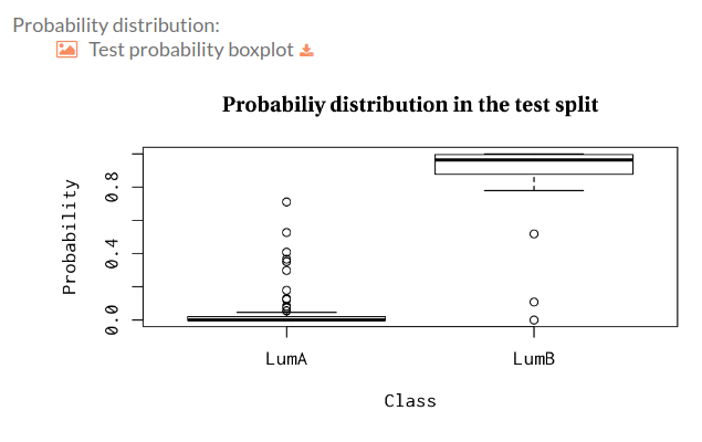
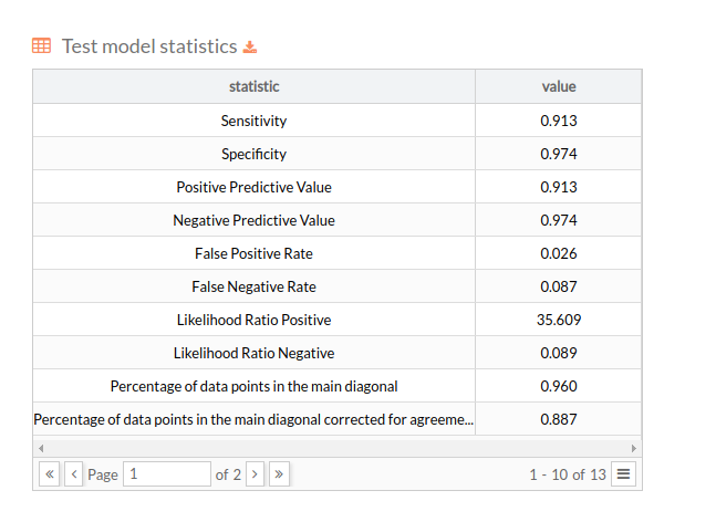
Then we show a table with the statistics of the model over the test set, in the same format as the one presented for the k-fold experiment. A well suited model for the problem at hand should not present a huge gap between the performance during the training and testing phases:
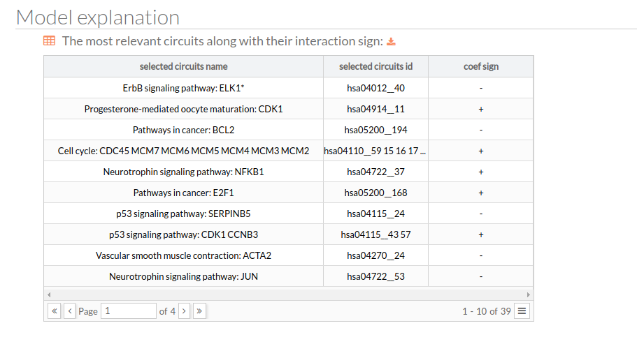
Model explanation
Here you will find a table with the most relevant circuits along with their interaction sign.
You can download the filtered circuits that best differentiate your phenotype. This section is only available when selecting Rank and filter circuits option.
Test report
When you select Use existing predictor you will have a different report for your test prediction study.
The test report is divided into four different panels:
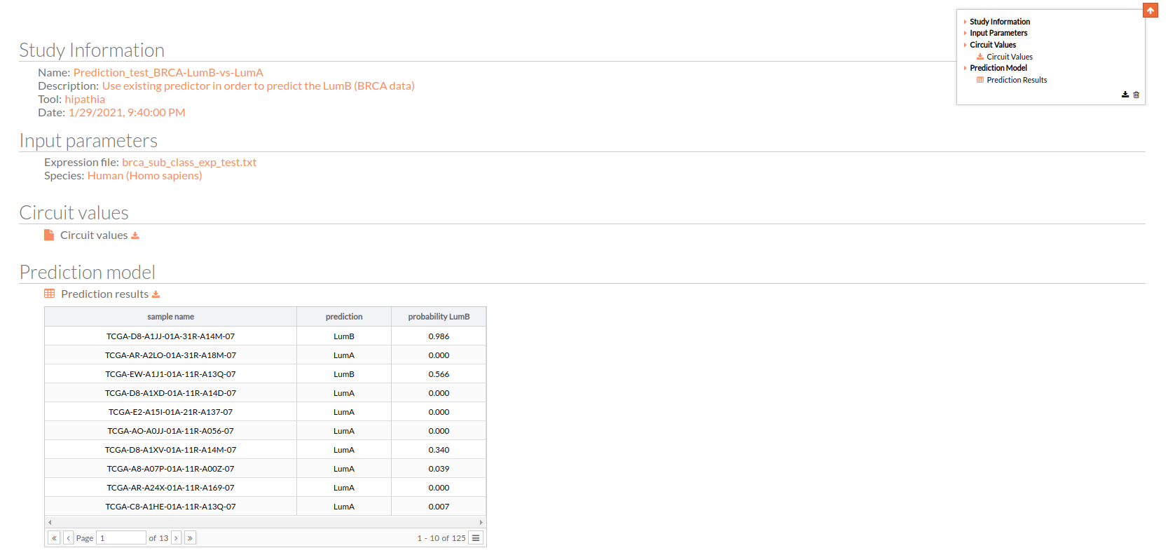
Study Information
As explained before, here you can find the information about the current study.
Input Parameters
The parameters with which the test study was launched, such as the name of the used expression file and the Species.
Circuit values
This matrix file indicates for each “effector circuit” the level of activation calculated using Hipathia method for each sample.
Prediction model
This is the most important result, this table is the predicted design file for your selected expression matrix using a previously trained model.
Workflow
The prediction tool is based on a machine learning module, this module of the Hipathia web tool can be summarized as follows:
- Expected input and output:
- Input features: hipathia circuit values.
- Input response: 1-D binary array with the same number of samples as the input features.
- Output 1: CV performance metrics
- Output 2: The selected features with their respective interaction sign, sorted by their relevance.
- A positive sign indicates that a given feature pushes the prediction towards the positive class.
- Output 3: Statistics and ROC, PR curves for typical train test split scenario.
- Output 4: Probability boxplots for the test set.
- Feature selection:
- We select the features that best discriminate between the response values by means of the LASSO [4] (using the
glmnetR package which implements a fast coordinate descent version of the LASSO [5]). - We filter the feature space using those circuits selected in the previous step.
- Hyperparameter search (
Ccost or margin and γ) of a non-linear SVM [6] with a radial-basis kernel:- γ: determines the complexity of the SVM frontier.
- cost: is basically the margin around the frontier established by the SVM.
- method: both γ and margin are obtained using a k-fold cross-validation procedure:
- for each selection of γ and
Cwe train a SVM - we compute the mean of the misclassification error over all the folds in the test split
- we select the best pair of hyperparameters (γ,
C), i.e. the ones with the lower CV mean error.
- From now onward we fix the features selected by the LASSO and the hyperparameters previously found.
- The SVM training has been carried out using the
LIBSVM[2] library by means of the R interface provided by the R packagee1071[1].
- Performance evaluation:
- We perform a k-fold cross-validation with the features and hyperparameters selected above in order to report the generalization capabilities of the method.
- The report contains a set of commonly used metrics for classification.
- We perform a train-test split analysis
- We randomly select 30% of the samples as the test
- We train a SVM on the train set using the hyperparameters and features previously found.
- We provide summary statistics as in the case of the k-fold cross-validation.
- We plot the ROC and Precision-Recall (PR) curves along with the area under the curve.
- Note that all curve visualizations have been done using the specialized R package
PRROC[3]
Bibliography
[1]D. Meyer, E. Dimitriadou, K. Hornik, A. Weingessel, and F. Leisch, e1071: Misc Functions of the Department of Statistics, Probability Theory Group (Formerly: E1071), TU Wien. 2019, https://CRAN.R-project.org/package=e1071
[2]C.-C. Chang and C.-J. Lin, “LIBSVM: A Library for Support Vector Machines,” ACM Trans. Intell. Syst. Technol., vol. 2, no. 3, pp. 27:1–27:27, May 2011, doi: 10.1145/1961189.1961199
[3]J. Grau, I. Grosse, and J. Keilwagen, “PRROC: computing and visualizing precision-recall and receiver operating characteristic curves in R,” Bioinformatics, vol. 31, no. 15, pp. 2595–2597, 2015, | doi: 10.1093/bioinformatics/btv153
[4]R. Tibshirani, “Regression Shrinkage and Selection via the Lasso,” Journal of the Royal Statistical Society. Series B (Methodological), vol. 58, no. 1, pp. 267–288, 1996, doi: 10.1111/j.2517-6161.1996.tb02080.x
[5]J. Friedman, T. Hastie, and R. Tibshirani, “Regularization Paths for Generalized Linear Models via Coordinate Descent,” J Stat Softw, vol. 33, no. 1, pp. 1–22, 2010, doi: 10.18637/jss.v033.i01
[6]C. Cortes and V. Vapnik, “Support-vector networks,” Mach Learn, vol. 20, no. 3, pp. 273–297, Sep. 1995, doi: 10.1007/BF00994018