
Table of Contents
Worked example prediction
The most common prediction problem in biomedicine is related to class membership assignation. That is, given two known classes of individuals, defined by their attributes (e.g. gene expression profile), a predictor would be able of taking a new, unknown individual, and assigning to it a probability of belonging to one of these classes using its attribute information.
The prediction is a two-step problem:
- Step 1: Training the predictor
- Step 2: Testing new samples.
The training phase is used to build the predictor. To do so, we need firstly a training set (a dataset of individuals belonging to two classes and properly labeled, or individuals with the associated measurement). This training set must be large and diverse enough to represent the real population of individuals on which we will be using the trained predictor. Then the predictor “learns” from this example training dataset how the classes are related to the attributes, which we will call features from now on. The performance is assessed by cross-validation, and several scores would give us an idea of how specific and sensible is the predictor. Once the predictor is trained and the performance is acceptable it is ready to be used. New samples can be tested with the predictor that will return a class membership probability.
It is important to note that, when the features used for training the predictor have a functional meaning by themselves, such as the signaling circuits have, the interpretation of the reasons for which the predictor takes a decision is straightforward and related to the biological processes that define the differences between the cases compared.
Below is a worked example of how to train and use a predictor/estimator/classifier. In this example, we will work with a subsample, those patients with a known molecular subtype of luminal A or luminal B, of the Breast Cancer dataset from the repository The Cancer Genome Atlas (TCGA) Link to dataset.
The example consists of predicting if a given sample is either luminal A or luminal B by learning a function that maps the signal activation values of a sample into the molecular classes. To simulate a real-world scenario where the trained estimator must classify unseen samples, we have built a train/test split of the chosen dataset. During the training phase, we only use the appropriately named train dataset, where the mapping function is learned. Then, the mapping function is applied to the holdout test set and the tool reports a series of useful classification metrics and plots along with the predicted molecular sub-types of the test samples. Note that during the training phase we also report the same set of metrics to infer the generalization capability of the learning method, when both sets of metrics are close we can conclude that the method has learned a useful mapping function.
Training: Build new predictor
In this example, we will work with the previously mentioned training split of the Breast Cancer dataset which consists of 335 luminal A and 170 luminal B samples. Follow the next steps in order to reproduce this worked example:
1- Log into HiPathia. For further information on this step visit logging in.
2- Collection of data. As we mentioned before, we will work with a Breast Cancer dataset from the repository The Cancer Genome Atlas (TCGA) Link to dataset.
More information on the proposed dataset is available here:
Before use in HiPathia, the dataset must be normalized. We recommend using the logarithm of the trimmed mean of M values (log2TMM).
We have selected samples of breast cancer tumors from the dataset, annotated as luminal A and luminal B (the molecular annotations come from this paper). You can learn more about breast cancer molecular subtypes here. The purpose of this study is to train a predictor so that it can learn to distinguish molecular subtypes from gene expression data using the Hipathia mechanistic models, and evaluate the model with a controlled set of samples.
The expression matrix and the experimental design can be downloaded from these links:
- Expression matrix: brca_sub_class_exp_train.txt
- Experimental design:brca_sub_class_des_train.txt
3- Click Prediction button.

4- Upload the normalized data to HiPathia by clicking My data in the data panel, or click the Run training example button. For further information on this step visit Upload your data.
 5- In the Type panel select Train new predictor.
6- In the Input data panel, select Expression matrix. Click the File browser of the Expression matrix section and select the desired file.

7- In the Design data panel, select Class predictor. Click the File browser of the Experimental design section and select the desired file. Automatically Condition 1 and Condition 2 files are selected. Select “Tumor” for Condition 1 and “Normal” for Condition 2.

8- Select Human (Homo sapiens) as species (default).
9- In the Pathways panel, select all the pathways (default).
10- In the Study information panel, click the File browser button and select the desired output folder. In this case, we will use analysis_BRCA. Give a name to the study, for example “BRCA train model”.

11- Click the Run analysis button. A Study will be created and listed in the studies panel. You can access this panel by clicking on the My studies button.
Training report
Once the launched study is finished, the report/results will be available in “My studies”. The report page of the Prediction-training tool includes different output results. You can download any table or image shown on the results page by clicking on the name right before it. You can also download the pathway and function matrices by clicking on Circuit values, For more information about each result please read Prediction - Training report and Prediction - Workflow sections.
Breast Cancer Molecular Subtype Classification
The experiment consists in classifying a given sample as Luminal A or Luminal B (molecular subtype). We use TCGA data, no pathway filtering was done by hand.
Model Analysis
CV Performance:
The most relevant features along with their interaction sign. It is important to note that, when the features used for training the predictor have a functional meaning by themselves, such as the signaling circuits have, the interpretation of the reasons for which the predictor takes a decision is straightforward and related to the biological processes that define the differences between the cases compared. The most relevant circuits with the interaction sign are:
| Selected circuits name | Coef sign |
| ErbB signaling pathway: ELK1* | - |
| Progesterone-mediated oocyte maturation: CDK1 | + |
| Pathways in cancer: BCL2 | - |
| Cell cycle: CDC45 MCM7 MCM6 MCM5 MCM4 MCM3 MCM2 | + |
| Neurotrophin signaling pathway: NFKB1 | + |
| Pathways in cancer: E2F1 | + |
| p53 signaling pathway: SERPINB5 | - |
| p53 signaling pathway: CDK1 CCNB3 | + |
| Vascular smooth muscle contraction: ACTA2 | - |
| Neurotrophin signaling pathway: JUN | - |
| Apoptosis: TP53 | + |
| PPAR signaling pathway: ACAA1 | - |
| Hippo signaling pathway: BIRC5 | + |
| PPAR signaling pathway: CPT1C | + |
| ErbB signaling pathway: GSK3B | + |
| cAMP signaling pathway: GRIN3A | + |
| Oocyte meiosis: CPEB2 | + |
| Pathways in cancer: CSF3R | + |
| Choline metabolism in cancer: WAS | + |
| NOD-like receptor signaling pathway: CASP5 | + |
| Hippo signaling pathway: SMAD1 SMAD4 | - |
| Pathways in cancer: BIRC5 | + |
| ErbB signaling pathway: STAT5A* | - |
| ErbB signaling pathway: STAT5A | - |
| p53 signaling pathway: CDK2 CCNE1 | + |
| Proteoglycans in cancer: MAPK1 | - |
| Pathways in cancer: CTBP1 HDAC1 | - |
| cGMP-PKG signaling pathway: CNGB1 | - |
| Ras signaling pathway: RAP1A | - |
| Oxytocin signaling pathway: EEF2 | - |
| Gap junction: C00681 | - |
| Insulin signaling pathway: G6PC | - |
| Fc gamma R-mediated phagocytosis: ARF6* | + |
| Platelet activation: PIK3R5* | - |
| Progesterone-mediated oocyte maturation: PIK3R5 | - |
| PI3K-Akt signaling pathway: CDKN1B | - |
| PPAR signaling pathway: FADS2 | + |
| Thyroid hormone signaling pathway: WNT4 | - |
| Thyroid hormone signaling pathway: CTNNB1 | - |
Split Analysis
Split Performance: Test stats
PR curve over the test:
 curve for the simulated test split.")
ROC curve over the test set:

Probability distributions of the positive class with respect to the true labels for the simulated test split:

Test: Use existing predictor
In this step, we will use the trained model in the previous step training of a model and testing it with a different split of the Breast Cancer dataset (125 Samples):
1. Log into HiPathia. For further information on this step visit Logging in.
2. Selection of test data: We have selected a different subset of the previous Breast Cancer dataset that were not used in the training of the model that we want to test.
You can download the expression matrix we use to test the model from this link:
- Test expression matrix: brca_sub_class_exp_test.txt
3- Click the Prediction button.
4- Upload the test data to HiPathia in the data panel by clicking My data, or click the Run test example button. For further information on this step visit Upload your data.
5- In the Type panel, select Test existing predictor. A window with all the existing models will appear. Select the model you want to use. The model information will appear on the right panel. You can follow the steps in Worked example Prediction - Train to train your own model with your data. We will test the model we have trained in that guided example.

6- In the Input data panel select Expression matrix. Click the File browser in the Expression matrix file section and select the desired file: brca_genes_vals_bn_test.txt.

7- In the Study information panel, click the File browser button and select the desired output folder. In this case, we will use analysis_BRCA. Give a name to the study, for example, “BRCA test model”.

8- Click the Run analysis button. A study will be created and listed in the studies panel. You can access this panel by clicking on the My studies button.
Test report
Once the launched study is finished, the report/results will be available in “My studies”. The report page of the Prediction-test tool includes different output results. You can download any table or image shown on the results page by clicking on the name right before it. For more information about each result please read Prediction - Test report and Prediction - Workflow sections.
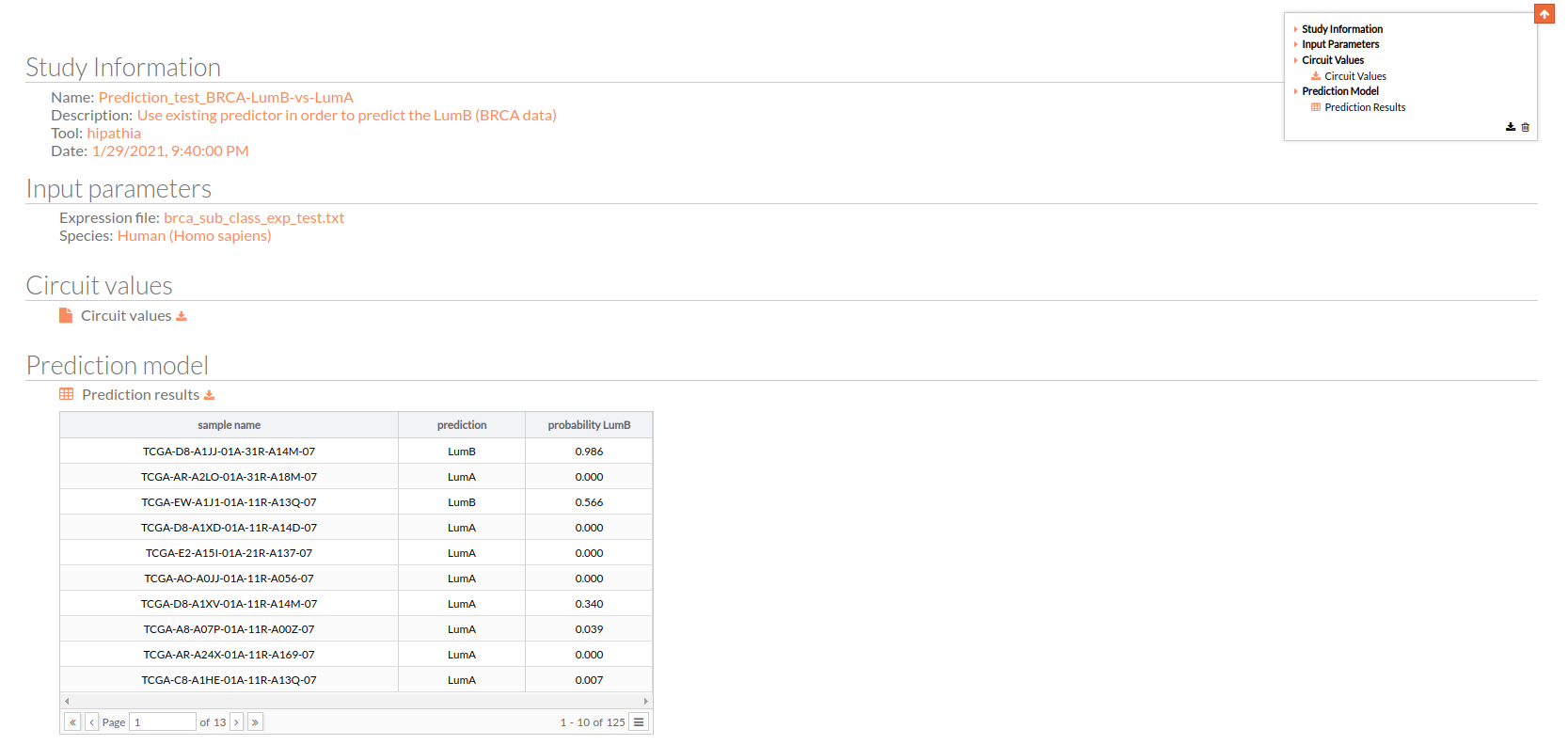
This is the most important result of our predictor, which is a matrix with three columns:
- Sample name: all the 125 samples (104 luminal A, 21 luminal B) in the used expression matrix file.
- Prediction: the predicted group LumB (Luminal B) or LumA (Luminal A)
- Probability LumB: this is the probability of being lumB, if it is 1 that means the predictor is 100% sure that the given result will be LumB.
You can download the matrix of predicted experimental design by clicking on Prediction results.
Prediction evaluation
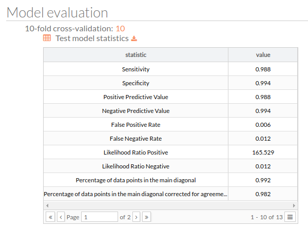
Note that for this example we know beforehand the ground truth labels so we can compute the classification metrics as in the simulated split during the training phase. The ROC and PR curves are quite similar to those of the simulated split which inform us of the good generalization capabilities of the tool for this problem. The trend can also be observed from the companion metrics table and the confusion matrix.


| statistic | value |
|---|---|
| Sensitivity | 0.761904761904762 |
| Specificity | 0.913461538461538 |
| Positive Predictive Value | 0.64 |
| Negative Predictive Value | 0.95 |
| False Positive Rate | 0.0865384615384616 |
| False Negative Rate | 0.238095238095238 |
| Likelihood Ratio Positive | 8.8042328042328 |
| Likelihood Ratio Negative | 0.260651629072682 |
| Percentage of data points in the main diagonal | 0.888 |
| Percentage of data points in the main diagonal corrected for agreement by chance | 0.627659574468085 |
| Rand index | 0.799483870967742 |
| Rand index corrected for agreement by chance | 0.525491509396793 |
| Total Accuracy | 0.888 |
| Reference | |||
|---|---|---|---|
| Lum A | LumB | ||
| Prediction | LumA | 95 | 5 |
| LumB | 9 | 16 | |
Discussion
There are huge clinical implications for being able to discern cancer types. Tumor classification in categories that respond to different kinds of treatments has the potential to help to target tumors with the most effective treatment options available for each type, greatly improving survival outcomes. Several years ago, the relevance of molecular subtyping in breast cancer was demonstrated, and from that moment, molecular profiling has been used as a tool to identify prognosis and risk predictors. An example of this approach is used, for example, in PAM50, MammaPrint, and OncoType DX predictions, widespread tools for breast cancer stratification and therapeutic strategy selection. Following these premises, we have tried to identify whether signaling circuits are as useful for cancer stratification and subtype prediction as gene expression values. The results suggest that, indeed, both gene expression and signaling activity can be used to differentiate between luminal A and luminal B breast tumors, showing the value of signaling activity measures as a predictive marker.
In this example, we introduce a machine learning workflow, a binary classification estimator fused with feature selection and normalization, built on top of the signalization circuit activation values, computed utilizing the HiPathia mechanistic model. The workflow has two main advantages over using the full gene set: on the one hand, the dimensionality of the feature space is amply compressed (thus filtering noise) since there are from ten, when using the full gene set, to three times fewer circuits than genes, if reducing the gene set to the signalization subset, and on the other hand, the machine learning model is more explainable due, among other things, to the use of a smaller set of features that in turn are easier to interpret thanks to the functional characterization of the circuits.
Our proposed experiment, consisting of differentiating between luminal breast cancer molecular subtypes, shows that our methodology is very suitable to this particular task, as can be inferred from the performance metrics computed on a fully independent set of samples and the CV splits. Furthermore, the excellent results are obtained using a small subset of the circuits, which reinforces the model explainability.
Related papers
Perou, C., Sørlie, T., Eisen, M. et al. Molecular portraits of human breast tumours. Nature 406, 747–752 (2000). https://doi.org/10.1038/35021093
Markopoulos C. Overview of the use of Oncotype DX(®) as an additional treatment decision tool in early breast cancer. Expert Rev Anticancer Ther. 2013 Feb;13(2):179-94. PMID: 23406559.https://doi.org/10.1586/era.12.174.
Caan BJ, Sweeney C, Habel LA, Kwan ML, Kroenke CH, Weltzien EK, Quesenberry CP Jr, Castillo A, Factor RE, Kushi LH, Bernard PS. Intrinsic subtypes from the PAM50 gene expression assay in a population-based breast cancer survivor cohort: prognostication of short- and long-term outcomes. Cancer Epidemiol Biomarkers Prev. 2014 May;23(5):725-34. Epub 2014 Feb 12. PMID: 24521998; PMCID: PMC4105204. https://doi.org/10.1158/1055-9965.EPI-13-1017.
The Cancer Genome Atlas Network., Genome sequencing centres: Washington University in St Louis., Koboldt, D. et al. Comprehensive molecular portraits of human breast tumours. Nature 490, 61–70 (2012). https://doi.org/10.1038/nature11412
Noske A, Anders S, Ettl J, Hapfelmeier A, Steiger K, Specht K et al. Risk stratification in luminal-type breast cancer: Comparison of Ki-67 with EndoPredict test results. The Breast. 2020;49:101-107. https://doi.org/10.1016/j.breast.2019.11.004.
Cancello G, Maisonneuve P, Rotmensz N, Viale G, Mastropasqua M, Pruneri G, et al. Progesterone receptor loss identifies Luminal B breast cancer subgroups at higher risk of relapse. Annals of Oncology. 2013;24(3):661-668. https://doi.org/10.1093/annonc/mds430.