
This is an old revision of the document!
Table of Contents
Worked example - Prediction
In this page we provide a walkthrough and a brief discussion of the Prediction tool. This comprises the training of a model and its testing with a different split of data.
Test inputs
1. Log into HiPathia. For further information on this step visit Logging in.
2. Selection of test data. We will work with a Breast Cancer dataset from the repository The Cancer Genome Atlas (TCGA) Link to dataset. More information on the original dataset is available here:
* https://www.nature.com/articles/nature11412
* https://pubmed.ncbi.nlm.nih.gov/23644459/
We have selected a subset of Breast Cancer samples from the dataset annotated as luminal A or luminal B (the molecular annotations come from this paper) that were not used in the training of the model that we want to test.
You can download the expression matrix we use to test the model from this link:
- Test expression matrix: brca_sub_class_exp_test.txt
3. Upload the test data to HiPathia in the data panel by clicking My data. For further information on this step visit Upload your data.
4. Click the Prediction button.

5. In the Type panel, select Test existing predictor. A window with all the existing models will appear. Select the model you want to use. The model information will appear on the right panel. You can follow the steps in Worked example Prediction - Train to train your own model with your data. We will test the model we have trained in that guided example.

6. In the Input data panel select Expression matrix. Click the File browser in the Expression matrix file section and select the desired file: brca_genes_vals_bn_test.txt.

7. In the Job information panel, click the File browser button and select the desired output folder. In this case, we will use analysis_BRCA. Give a name to the study, for example, “BRCA test model”.

8. Click the Run analysis button. A study will be created and listed in the studies panel. You can access this panel by clicking on the My studies button.
Test report
This section provides a walkthrough of the report page generated when testing a previously trained model with another split of data.
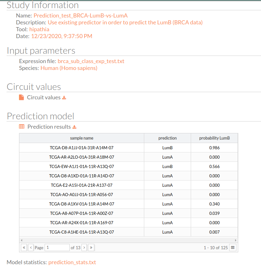
Study Information
Here appears the information about the selected study.
- Name: the study name.
- Description: the description of the current study.
- Tool: the name of the used tool (in this case, is Hipathia).
- Date: study's launching date (MM/DD/AAAA, HH:MM:SS AM/PM format)
Input Parameters
Here appear the parameters with which the current study was launched.

- Expression file: The name of the expression file that has been used in the current study.
- Species: The species of this experiment; Human (Homo sapiens), Mouse (Mus musculus), or Rat (Rattus norvegicus).
Circuit values
The matrix of circuit activity values can be downloaded by clicking circuit values. This matrix file indicates for each “effector circuit” the level of activation calculated using the HiPathia method for each sample.
Prediction model
This is the most important result of our predictor, which is a matrix with three columns:
- Sample name: all the 125 samples in the used expression matrix file.
- Prediction: the predicted group LumB (Luminal B) or LumA (Luminal A)
- Probability LumB: this is the probability of being lumB, if it is 1 that means the predictor is 100% sure that the given result will be LumB.
You can download the matrix of predicted experimental design by clicking on Prediction results.
Prediction evaluation
Confusion Matrix and Statistics
| Reference | |||
|---|---|---|---|
| Lum A | LumB | ||
| Prediction | LumA | 95 | 5 |
| LumB | 9 | 16 | |
| Accuracy | 0.888 | ||
|---|---|---|---|
| 95% CI | (0.8192, 0.9374) | ||
| No Information Rate | 0.832 | ||
| P-Value [Acc > NIR] | 0.0547 | ||
| Kappa | 0.6277 | ||
| Mcnemar's Test | |||
|---|---|---|---|
| P-Value | 0.4227 | ||
| Sensitivity | 0.9135 | ||
| Specificity | 0.7619 | ||
| Pos Pred Value | 0.9500 | ||
| Neg Pred Value | 0.6400 | ||
| Prevalence | 0.8320 | ||
| Detection Rat | 0.7600 | ||
| Detection Prevalence | 0.8000 | ||
| Balanced Accuracy | 0.8377 | ||
Discussion
There are huge clinical implications for being able to discern cancer types. Tumor classification in categories that respond to different kinds of treatments has the potential to help to target tumors with the most effective treatment options available for each type, greatly improving survival outcomes. Several years ago, the relevance of molecular subtyping in breast cancer was demonstrated, and from that moment, molecular profiling has been used as a tool to identify prognosis and risk predictors [1]. An example of this approach is used, for example, in PAM50, MammaPrint, and OncoType DX predictions, widespread tools for breast cancer stratification and therapeutic strategy selection. Following these premises, we have tried to identify whether signaling circuits are as useful for cancer stratification and subtype prediction as gene expression values. The results suggest that, indeed, both gene expression and signaling activity can be used to differentiate between luminal A and luminal B breast tumors, showing the value of signaling activity measures as a predictive marker.
In this example we introduce a machine learning workflow, a binary classification estimator fused with feature selection and normalization, built on top of the signalization circuit activation values, computed utilizing the HiPathia mechanistic model. The workflow has two main advantages over using the full gene set: on the one hand, the dimensionality of the feature space is amply compressed (thus filtering noise) since there are from ten, if using the full gene set, to three times fewer circuits than genes, if reducing the gene set to the signalization subset, and on the other hand, the machine learning model is more explainable due, among other things, to the use of a smaller set of features that in turn are easier to interpret thanks to the functional characterization of the circuits.
Our proposed experiment, consisting of differentiating between luminal breast cancer molecular subtypes, shows that our methodology is very suitable to this particular task, as can be inferred from the performance metrics computed on a fully independent set of samples and the CV splits. Furthermore, the excellent results are obtained using a small subset of the circuits, which reinforces the model explainability.
Related papers
[1] Perou, C., Sørlie, T., Eisen, M. et al. Molecular portraits of human breast tumours. Nature 406, 747–752 (2000). https://doi.org/10.1038/35021093
Markopoulos C. Overview of the use of Oncotype DX(®) as an additional treatment decision tool in early breast cancer. Expert Rev Anticancer Ther. 2013 Feb;13(2):179-94. PMID: 23406559.https://doi.org/10.1586/era.12.174.
Caan BJ, Sweeney C, Habel LA, Kwan ML, Kroenke CH, Weltzien EK, Quesenberry CP Jr, Castillo A, Factor RE, Kushi LH, Bernard PS. Intrinsic subtypes from the PAM50 gene expression assay in a population-based breast cancer survivor cohort: prognostication of short- and long-term outcomes. Cancer Epidemiol Biomarkers Prev. 2014 May;23(5):725-34. Epub 2014 Feb 12. PMID: 24521998; PMCID: PMC4105204. https://doi.org/10.1158/1055-9965.EPI-13-1017.
The Cancer Genome Atlas Network., Genome sequencing centres: Washington University in St Louis., Koboldt, D. et al. Comprehensive molecular portraits of human breast tumours. Nature 490, 61–70 (2012). https://doi.org/10.1038/nature11412
Noske A, Anders S, Ettl J, Hapfelmeier A, Steiger K, Specht K et al. Risk stratification in luminal-type breast cancer: Comparison of Ki-67 with EndoPredict test results. The Breast. 2020;49:101-107. https://doi.org/10.1016/j.breast.2019.11.004.
Cancello G, Maisonneuve P, Rotmensz N, Viale G, Mastropasqua M, Pruneri G et al. Progesterone receptor loss identifies Luminal B breast cancer subgroups at higher risk of relapse. Annals of Oncology. 2013;24(3):661-668. https://doi.org/10.1093/annonc/mds430.