
This is an old revision of the document!
Table of Contents
Worked example Prediction
Training
1- Log into HiPathia. For further information on this step visit logging in.
2- Collection of data. We will work with a Breast Cancer dataset from the repository The Cancer Genome Atlas (TCGA) Link to dataset.
More information on the proposed dataset is available here:
Before use in HiPathia, the dataset must be normalized. We recommend using the logarithm of the trimmed mean of M values (log2TMM).
We have selected samples of breast cancer tumors from the dataset, annotated as luminal A and luminal B (the molecular annotations come from this paper). You can learn more about breast cancer molecular subtypes here. The purpose of this study is to train a predictor so that it can learn to distinguish molecular subtypes from gene expression data using the Hipathia mechanistic models, and evaluate the model with a controlled set of samples.
The expression matrix and the experimental design can be downloaded from these links:
- Expression matrix: brca_sub_class_exp_train.txt
- Experimental design:brca_sub_class_des_train.txt
3- Click Prediction button.

4- Upload the normalized data to HiPathia by clicking My data in the data panel, or click the Run training example button. For further information on this step visit Upload your data.
 5. In the Type panel select Train new predictor.
6. In the Input data panel, select Expression matrix. Click the File browser of the Expression matrix section and select the desired file.

7. In the Design data panel, select Class predictor. Click the File browser of the Experimental design section and select the desired file. Automatically Condition 1 and Condition 2 files are selected. Select “Tumor” for Condition 1 and “Normal” for Condition 2.

8. Select Human (Homo sapiens) as species (default).
9. In the Pathways panel, select all the pathways (default).
10. In the Study information panel, click the File browser button and select the desired output folder. In this case, we will use analysis_BRCA. Give a name to the study, for example “BRCA train model”.

11. Click the Run analysis button. A Study will be created and listed in the studies panel. You can access this panel by clicking on the My studies button.
Training report
Once the launched study is finished, the report/results will be available in “My studies”. The report page of the Prediction-training tool includes different output results. You can download any table or image shown on the results page by clicking on the name right before it. You can also download the pathway and function matrices by clicking on Circuit values, For more information about each result please read Prediction - Training report section.
Input Parameters
Here you can visualize the parameters with which the current study was launched.
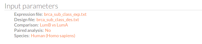
- Expression file: The name of the expression file that has been used in the current study.
- Design file: The name of the design file that has been used in the current study.
- Comparison: The groups that have been compared, for example; Normal vs Tumor.
- Paired analysis: Have the input data been paired? No or Yes.
- Species: The species of this experiment; Human (Homo sapiens), Mouse (Mus musculus) or Rat (Rattus norvegicus).
Circuit values
You can download the matrix of circuit activity values by clicking on circuit values.
 This matrix file indicates for each “effector circuit” the level of activation calculated using Hipathia method for each sample.
Model training
Here you can visualize the results from the prediction analysis.
- K-fold cross-validation: The number of equal sized subsamples in which the original sample is randomly partitioned.
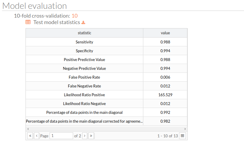
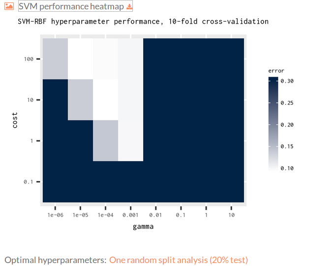
- SVM-RBF hypermeter performance
- Test model statistics:
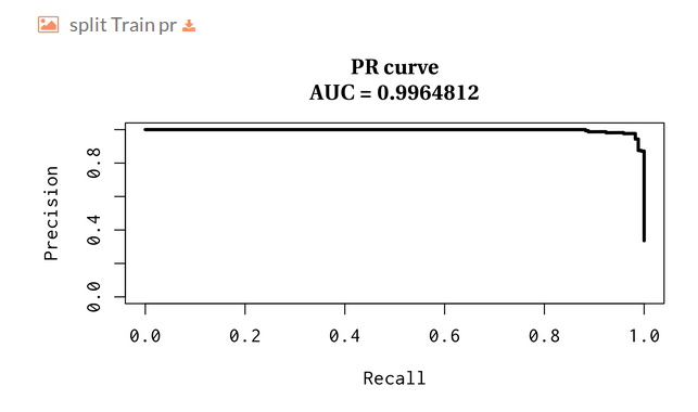
- Split Train pr:
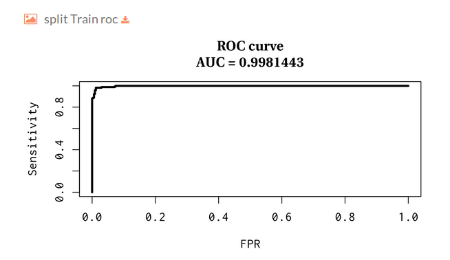
- Split Train roc:
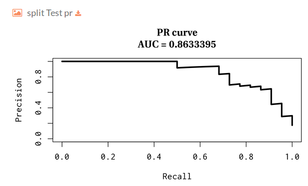
- Split Test pr:
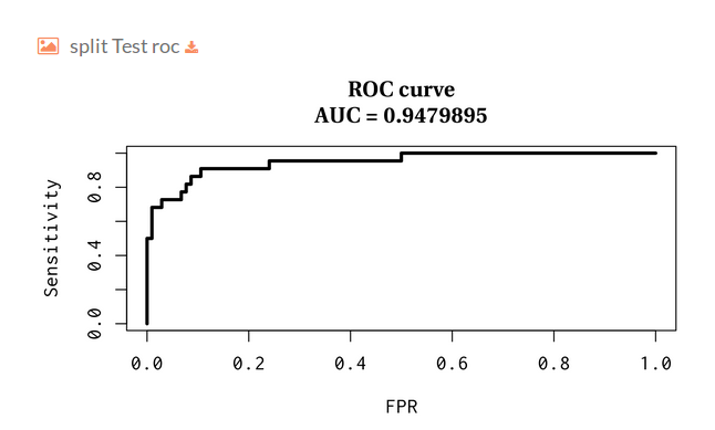
- Split Test roc:
Prediction model
Model statistics
You can download the model statistics.
- Selected features: You can download the filtered paths that best differentiate your phenotype. This section is only available when selecting filter paths option.
Workflow
The prediction tool is based on a machine learning module, this module of the Hipathia web tool can be summarized as follows:
- Expected input and output:
- Input features: Hipathia circuit values.
- Input response: 1-D binary array with the same number of samples as the input features.
- Output 1: CV performance metrics
- Output 2: The selected features with their respective interaction sign, sorted by their relevance.
- A positive sign indicates that a given feature pushes the prediction towards the positive class.
- Output 3: Statistics and ROC, PR curves for typical train test split scenario.
- Output 4: Probability boxplots for the test set.
- Feature selection:
- We select the features that best discriminate between the response values by means of the LASSO [4] (using the
glmnetr package which implements a fast coordinate descent version of the LASSO [5]). - We filter the feature space using those circuits selected in the previous step.
- Hyperparameter search (
Ccost or margin and γ) of a non-linear SVM [6] with a radial-basis kernel:- γ: determines the complexity of the svm frontier.
- cost: is basically the margin around the frontier established by the svm.
- method: both γ and margin are obtained using a k-fold cross-validation procedure:
- for each selection of γ and
Cwe train a svm - we compute the mean of the misclassification error over all the folds in the test split
- we select the best pair of hyperparameters (γ,
C), i.e. the ones with the lower CV mean error.
- From now onwards we fix the features selected by the LASSO and the hyperparameters previously found.
- The
SVMtraining has been carried out using theLIBSVMlibrary [2] by means of the R interface provided by the packagee1071[1].
- Performance evaluation:
- We perform a k-fold cross-validation with the features and hyperparameters selected above in order to report the generalization capabilities of the method.
- The report contains a set of commonly used metrics for classification.
- We perform a train-test split analysis
- We randomly select 30% of the samples as the test
- We train a SVM on the train set using the hyperparameters and features previously found.
- We provide summary statistics as in the case of the k-fold cross-validation.
- We plot the ROC and Precision-Recall (PR) curves along with the area under the curve.
- Note that all curve visualizations have been done using the specialized R package
PRROC[3]
Breast Cancer Molecular Subtype Classification
The experiment consists in classifying a given sample as Luminal A or Luminal B (molecular subtype). We use TCGA data, no pathway filtering was done by hand.
Model Analysis
Hyperparameter search:

CV Performance: CV stats
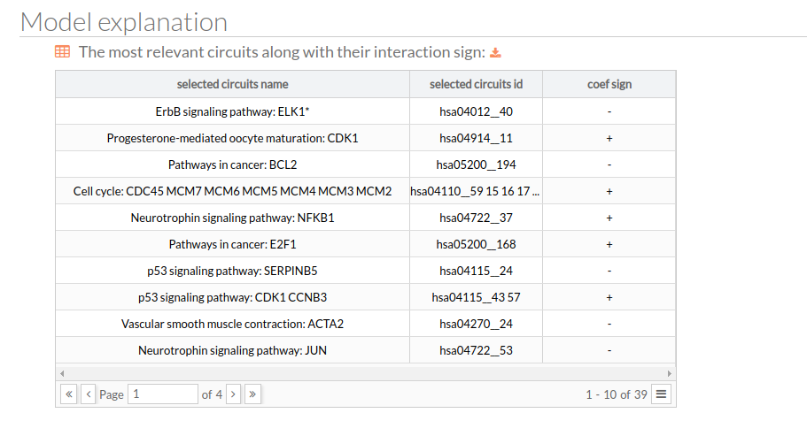
The most relevant features along with their interaction sign:
| features | coefs |
| p53 signaling pathway: CDK1 CCNB3 | + |
| p53 signaling pathway: CDK2 CCNE1 | + |
| p53 signaling pathway: SERPINB5 | - |
| Oocyte meiosis: REC8* | + |
| Neurotrophin signaling pathway: NFKB1 | + |
| Neurotrophin signaling pathway: RHOA | + |
| Amphetamine addiction: ARC | - |
| RIG-I-like receptor signaling pathway: CHUK IKBKB IKBKG | + |
| Ras signaling pathway: RAP1A | - |
| Progesterone-mediated oocyte maturation: CDK1 | + |
| Vascular smooth muscle contraction: ACTA2 | - |
| Complement and coagulation cascades: BDKRB1 | + |
| Fanconi anemia pathway: RAD51C | + |
| TGF-beta signaling pathway: ROCK1 | - |
| ErbB signaling pathway: ELK1* | - |
| HTLV-I infection: TP53 TBPL2 | + |
| Platelet activation: ITPR1 | - |
| Pathways in cancer: E2F1 | + |
| PI3K-Akt signaling pathway: BCL2 | - |
| Maturity onset diabetes of the young: NKX6-1 | + |
| Signaling pathways regulating pluripotency of stem cells: MAPK1* | - |
| Rap1 signaling pathway: THBS1 | + |
| HTLV-I infection: E2F1 | + |
| Jak-STAT signaling pathway: CDKN1A | + |
| Epstein-Barr virus infection: RB1 | - |
| Colorectal cancer: BIRC5 | + |
| Signaling pathways regulating pluripotency of stem cells: MYC | - |
| Taste transduction: C00076* | - |
| Hepatitis B: JUN | - |
| Axon guidance: GSK3B | - |
| MAPK signaling pathway: MAPT | - |
| cAMP signaling pathway: HHIP | - |
| Fanconi anemia pathway: BRCA1 | + |
| Pathways in cancer: CSF3R | + |
| Cell cycle: CDC45 MCM7 MCM6 MCM5 MCM4 MCM3 MCM2 | + |
| ErbB signaling pathway: CDKN1A | + |
| HTLV-I infection: PTTG2 | + |
| AMPK signaling pathway: CCNA2 | + |
| Oocyte meiosis: CDC25C* | + |
| Non-alcoholic fatty liver disease (NAFLD): BAX | + |
| Hepatitis B: PCNA | + |
| AMPK signaling pathway: G6PC | - |
| Adrenergic signaling in cardiomyocytes: BCL2 | - |
| HTLV-I infection: ANAPC10 CDC20 | - |
| Progesterone-mediated oocyte maturation: CDK1* | + |
| Complement and coagulation cascades: C4A | - |
| Choline metabolism in cancer: WAS | + |
| ErbB signaling pathway: STAT5A | - |
| Herpes simplex infection: FOS | - |
| Amyotrophic lateral sclerosis (ALS): DERL1 | + |
| AGE-RAGE signaling pathway in diabetic complications: F3 | - |
| Non-alcoholic fatty liver disease (NAFLD): PKLR | + |
| Maturity onset diabetes of the young: FOXA3 | - |
| AMPK signaling pathway: CPT1C | + |
| PPAR signaling pathway: FADS2 | + |
| Rap1 signaling pathway: C00076* | + |
| cAMP signaling pathway: GRIN3A | + |
| Glutamatergic synapse: CACNA1A | - |
| Progesterone-mediated oocyte maturation: MAPK14 | - |
| Salivary secretion: BEST2 | + |
| Vibrio cholerae infection: PDIA4 | + |
| cAMP signaling pathway: PLN | + |
| Neurotrophin signaling pathway: JUN | - |
| Pathways in cancer: CCNA1 | - |
| Epithelial cell signaling in Helicobacter pylori infection: GIT1 | - |
| Renal cell carcinoma: TGFA | - |
| Influenza A: RNASEL | + |
| Thyroid hormone signaling pathway: TP53* | + |
| Epithelial cell signaling in Helicobacter pylori infection: CXCL1 | - |
| Signaling pathways regulating pluripotency of stem cells: MAPK14 | + |
| Hepatitis C: EIF2S1 | + |
| Proteoglycans in cancer: CTNNB1 | + |
| Influenza A: STAT1 IRF9 | + |
| Thyroid hormone signaling pathway: CTNNB1 | - |
| Taste transduction: PKD1L3 PKD2L1 | + |
| Prostate cancer: C16038 | - |
| Basal cell carcinoma: PTCH1* | - |
| Toxoplasmosis: C06314 | - |
| Prostate cancer: BCL2 | - |
| Measles: EIF2S1 | + |
| Acute myeloid leukemia: CCNA1 | - |
| Glucagon signaling pathway: CPT1C* | + |
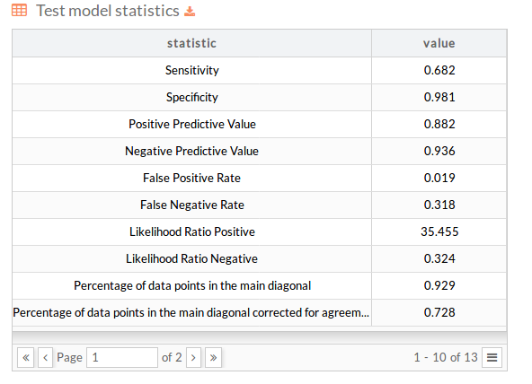
Split Analysis
Split Performance: Test stats
PR curve over the test:
 curve for the test split.")
ROC curve over the test set:

Probability for the test set:

Bibliography
[1]D. Meyer, E. Dimitriadou, K. Hornik, A. Weingessel, and F. Leisch, e1071: Misc Functions of the Department of Statistics, Probability Theory Group (Formerly: E1071), TU Wien. 2019, https://CRAN.R-project.org/package=e1071
[2]C.-C. Chang and C.-J. Lin, “LIBSVM: A Library for Support Vector Machines,” ACM Trans. Intell. Syst. Technol., vol. 2, no. 3, pp. 27:1–27:27, May 2011, doi: 10.1145/1961189.1961199.
[3]J. Grau, I. Grosse, and J. Keilwagen, “PRROC: computing and visualizing precision-recall and receiver operating characteristic curves in R,” Bioinformatics, vol. 31, no. 15, pp. 2595–2597, 2015, doi: 10.1093/bioinformatics/btv153
[4]R. Tibshirani, “Regression Shrinkage and Selection via the Lasso,” Journal of the Royal Statistical Society. Series B (Methodological), vol. 58, no. 1, pp. 267–288, 1996, doi: 10.1111/j.2517-6161.1996.tb02080.x
[5]J. Friedman, T. Hastie, and R. Tibshirani, “Regularization Paths for Generalized Linear Models via Coordinate Descent,” J Stat Softw, vol. 33, no. 1, pp. 1–22, 2010, doi: 10.18637/jss.v033.i01
[6]C. Cortes and V. Vapnik, “Support-vector networks,” Mach Learn, vol. 20, no. 3, pp. 273–297, Sep. 1995, doi: 10.1007/BF00994018.